
I think it’s fair to say that most academics who learn about R do so in the process of training or applying quantitative research methods. As a consequence, knowledge of R among academics tends to be limited to core (base) R packages (R Core Team, 2018) and a small handful of speciality statistical packages, e.g., {lavaan}, {lme4}, {MASS}, {car}, etc. With this in mind, the goal of this post is to provide an overview of three things to know beyond base R.
A more appropriate title for this post could be, “A quick introduction to the tidyverse,” as all of the following things to know beyond base R come from the {tidyverse}–a collection of high-powered, consistent, and easy-to-use packages developed by a number of thoughtful and talented R developers, so this should really be considered an exceptionally brief introduction to parts of the tidyverse. But users don’t need to know know everything about the tidyverse to reap the benefits of it. However, if you’re interested in a more formal/thorough introduction to the tidyverse, I would strongly encourage you to checkout R for Data Science by Garrett Groleman and Hadley Wickham.
For those of you who still might be hestitant about moving beyond base R, consider the plot below, which shows the download counts of {tidyverse} packages compared to several well-known and highly-regarded statistical packages.
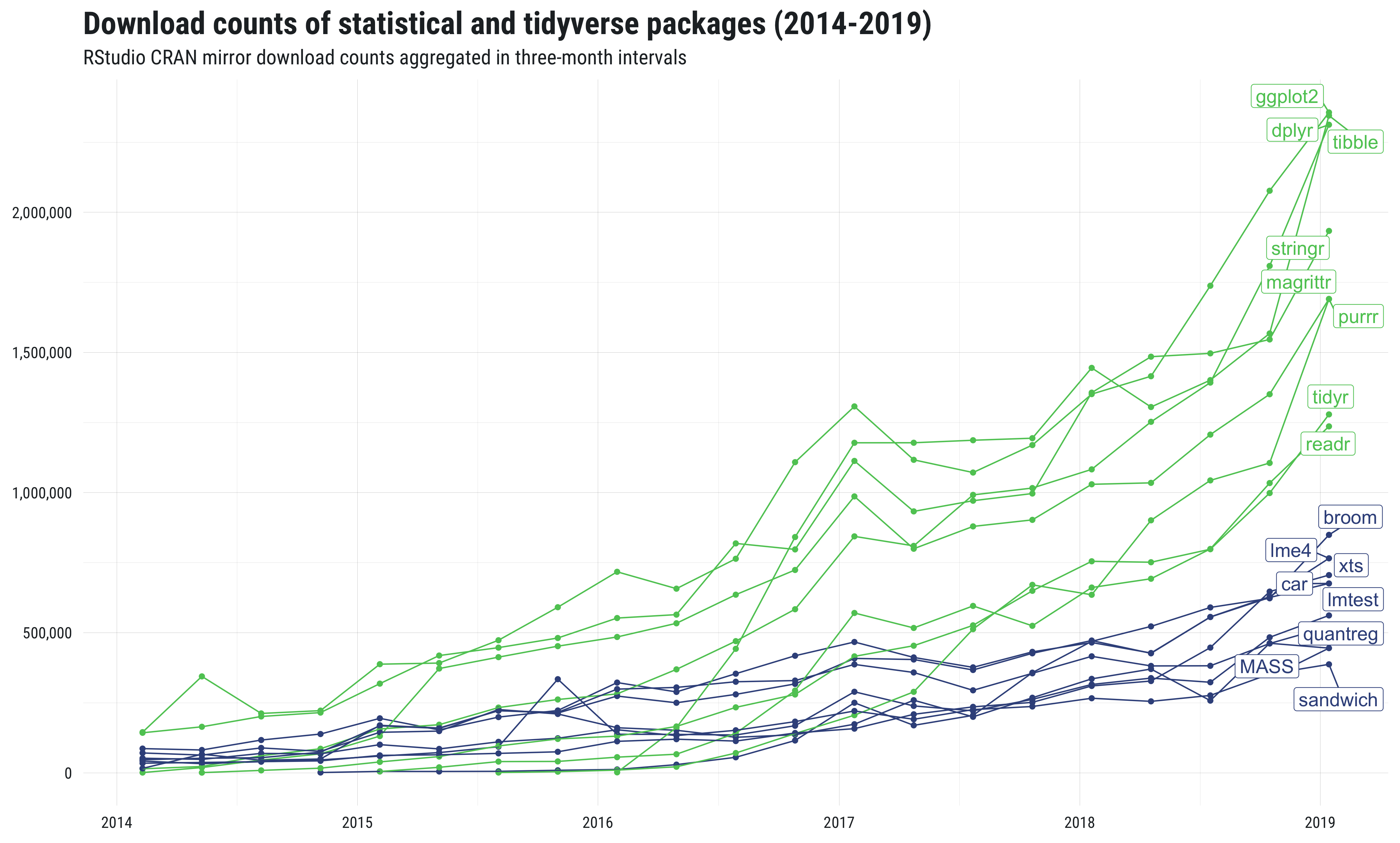
This plot hopefully demonstrates two things. First, that a lot of people use (and therefore test, troubleshoot, and write documentation for) tidyverse packages. Second, that use of tidyverse packages is not merely a fad or momentary trend. Indeed, compared to widely used statistical packages, there is a considerably higher download rate among tidyverse packages (even above and beyond the general uptick in overall R usage).
1. The pipe
The first thing to know beyond base R is the pipe. The pipe refers to the
%>% operator from the {magrittr} package.
library(magrittr)It may seem complicated at first, but what the pipe does is actually quite simple. That is, it allows users to write linear code. To illustrate use of the pipe, consider the following code that takes the mean of the log of three numbers:
mean(log(c(1, 3, 9)))
#> [1] 1.098612
Notice how the numbers c(1, 3, 9) are nested inside log(), which is then nested inside
mean()? If you’re reading the code from left-to-right, it means the functions are performed in
reverse order from how they are written. If we broke the code down into its three functions, we would
actually expect the order of operations to proceed as follows:
- Concacenate numbers into vector
c(...) - Log the numeric vector
log(...) - Estimate the mean of the logged numeric vector
mean(...)
With this order in mind, now consider the following piped code, which takes a numeric vector
c(1, 3, 9), calculates the log(), and then estimates the mean(). Hopefully
you notice that, in contrast to the nested code above, the code below is linear; in other words, the code appears in
the same order (moving from left to right) as the operations are performed.
c(1, 3, 9) %>% log() %>% mean()
#> [1] 1.098612
As a convention designed to make piped code even easier to read, users are encouraged to place each piped statement on its own line. So the code above should be rewritten as follows:
c(1, 3, 9) %>%
  log() %>%
  mean()
#> [1] 1.098612
2. The tibble
R is my favorite programming language because nearly everyone who uses it either works with data
frames or is extremely familiar with them. With all of the use and attention, it is hardly surprising
that there would be some improvements to the traditional data.frame, which is why the
tibble is the second thing to know beyond base R. The tibble refers to a data frame-like class
produced by the {tibble} package. Tibbles (class tbl_df) are
essentially a special variant of data frames that have desirable properties for printing and joining. And because
they also inherit the data.frame class, they also behave like data frames 99.9% (and, seriously, I
wouldn’t worry about the 0.1%).
As the code illustrates below, it’s easy to convert nearly any data frame into a tibble via
tibble::as_tibble():
(mtcars <- tibble::as_tibble(mtcars))
#> # A tibble: 32 x 11
#>     mpg   cyl  disp    hp  drat    wt  qsec    vs    am  gear  carb
#>   <dbl> <dbl> <dbl> <dbl> <dbl> <dbl> <dbl> <dbl> <dbl> <dbl> <dbl>
#> 1  21       6   160   110  3.9   2.62  16.5     0     1     4     4
#> 2  21       6   160   110  3.9   2.88  17.0     0     1     4     4
#> 3  22.8     4   108    93  3.85  2.32  18.6     1     1     4     1
#> 4  21.4     6   258   110  3.08  3.22  19.4     1     0     3     1
#> 5  18.7     8   360   175  3.15  3.44  17.0     0     0     3     2
#> # … with 27 more rows
It’s also possible to create tibbles directly via tibble::tibble(...), e.g.,
tibble::tibble(
  x = rnorm(100),
  y = rnorm(100),
  z = sample(letters, 100, replace = TRUE)
)
#> # A tibble: 100 x 3
#>       x      y z
#>   <dbl>  <dbl> <chr>
#> 1 0.138  0.851 u
#> 2 0.894 -0.295 m
#> 3 0.377  1.61  u
#> 4 0.345 -0.332 r
#> 5 0.508  1.24  m
#> # … with 95 more rows
You hopefully noticed in the printing of the two previous code chunks that tibbles print out a lot prettier than normal data frames. Each observations is limited to a single line (no horizontal scrolling or wrapping). Not all rows are printed by default. And the printout also includes meta information about the classes of variables and the number of rows and columns and in the data set.
If you were really paying attention, you may have also noticed the z variable in the tibble built from
scratch was stored (by default) as a character vector and not a factor. This is another
important difference in tibbles compared to data frames. Tibbles are lazy, which is this case is useful for avoiding
join or mutate errors later on related to a limited set of observed factor levels.
3. Select, filter, arrange, and mutate
If I could only use one package beyond base R, it’d probably be {dplyr}, which is why key dplyr functions are the third thing to learn beyond base R. Compared to base R, the beauty of these {dplyr} functions is that they feature consistent design principles, easily work with non-standard evaluation (i.e., you don’t have to put quotes around variable names), and even leverage c++ behind the scenes for improved performance.
{dplyr} has tons of useful features, but its fundamental building blocks allow users to select columns,
dplyr::select(mtcars, cyl, wt, mpg, gear)
#> # A tibble: 32 x 4
#>     cyl    wt   mpg  gear
#>   <dbl> <dbl> <dbl> <dbl>
#> 1     6  2.62  21       4
#> 2     6  2.88  21       4
#> 3     4  2.32  22.8     4
#> 4     6  3.22  21.4     3
#> 5     8  3.44  18.7     3
#> # … with 27 more rows
mutate columns (i.e., transform, add),
mtcars %>%
  dplyr::mutate(mpg_per_cyl = mpg / cyl,
    car = row.names(datasets::mtcars)) %>%
  dplyr::select(car, mpg, cyl, mpg_per_cyl)
#> # A tibble: 32 x 4
#>   car                 mpg   cyl mpg_per_cyl
#>   <chr>             <dbl> <dbl>       <dbl>
#> 1 Mazda RX4          21       6        3.5
#> 2 Mazda RX4 Wag      21       6        3.5
#> 3 Datsun 710         22.8     4        5.7
#> 4 Hornet 4 Drive     21.4     6        3.57
#> 5 Hornet Sportabout  18.7     8        2.34
#> # … with 27 more rows
filter rows,
dplyr::filter(mtcars, cyl == 4, mpg >= 10)
#> # A tibble: 11 x 11
#>     mpg   cyl  disp    hp  drat    wt  qsec    vs    am  gear  carb
#>   <dbl> <dbl> <dbl> <dbl> <dbl> <dbl> <dbl> <dbl> <dbl> <dbl> <dbl>
#> 1  22.8     4 108      93  3.85  2.32  18.6     1     1     4     1
#> 2  24.4     4 147.     62  3.69  3.19  20       1     0     4     2
#> 3  22.8     4 141.     95  3.92  3.15  22.9     1     0     4     2
#> 4  32.4     4  78.7    66  4.08  2.2   19.5     1     1     4     1
#> 5  30.4     4  75.7    52  4.93  1.62  18.5     1     1     4     2
#> # … with 6 more rows
and arrange rows.
dplyr::arrange(mtcars, dplyr::desc(mpg))
#> # A tibble: 32 x 11
#>     mpg   cyl  disp    hp  drat    wt  qsec    vs    am  gear  carb
#>   <dbl> <dbl> <dbl> <dbl> <dbl> <dbl> <dbl> <dbl> <dbl> <dbl> <dbl>
#> 1  33.9     4  71.1    65  4.22  1.84  19.9     1     1     4     1
#> 2  32.4     4  78.7    66  4.08  2.2   19.5     1     1     4     1
#> 3  30.4     4  75.7    52  4.93  1.62  18.5     1     1     4     2
#> 4  30.4     4  95.1   113  3.77  1.51  16.9     1     1     5     2
#> 5  27.3     4  79      66  4.08  1.94  18.9     1     1     4     1
#> # … with 27 more rows
Chain these {dplyr} functions together with the pipe operator %>% to achieve linear/tidyverse-style
coding excellence.
mtcars %>%
  dplyr::filter(gear == 4) %>%
  dplyr::mutate(wt_mpg = wt / mpg) %>%
  dplyr::select(cyl, wt, mpg, wt_mpg) %>%
  dplyr::arrange(wt_mpg)
#> # A tibble: 12 x 4
#>     cyl    wt   mpg wt_mpg
#>   <dbl> <dbl> <dbl>  <dbl>
#> 1     4  1.62  30.4 0.0531
#> 2     4  1.84  33.9 0.0541
#> 3     4  2.2   32.4 0.0679
#> 4     4  1.94  27.3 0.0709
#> 5     4  2.32  22.8 0.102
#> # … with 7 more rows